Transmission Line Types in High-Speed PCB Layout

High-speed design is often described as if it starts at some magic clock frequency, but frequency is not what matters. What matters is whether the edge of the signal is fast enough and the trace long enough that the conductor behaves like a transmission line. Once that happens, the trace has an impedance, the return path is part of the circuit, and layout decisions that were previously cosmetic become electrical. Understanding the transmission line types used in PCB layout is the starting point for getting those decisions right.

When a Trace Becomes a Transmission Line

A short trace at a low frequency behaves as a simple conductor: the voltage at the far end is essentially the voltage at the near end, and the delay is irrelevant. As the edge rate increases and the trace lengthens, the propagation delay becomes comparable to the rise time, and the waveform no longer fits in the trace. Reflections appear at the ends, and the received signal shows overshoot, ringing and a delayed threshold crossing. These are the classic signal integrity symptoms of an uncontrolled transmission line.

A practical test is to compare the rise time with the one-way propagation delay. When the trace delay is a significant fraction of the rise time, the trace should be treated as a transmission line. Any signal with a rise time of about 5 ns or less falls into this class, and a device can generate fast edges even when its clock is slow, so the clock frequency alone is a poor guide.

Microstrip and Stripline

A transmission line consists of a signal conductor and its return path, separated by dielectric. In a microstrip, the signal runs on an outer layer with a reference plane on the layer beneath, and part of the field travels in air above the trace. That mixed dielectric makes the impedance sensitive to solder mask thickness and surface conditions, but microstrip is easy to route and easy to probe.

In a stripline, the signal is buried between two reference planes. The field is entirely inside the laminate, so the impedance is more stable and radiation is lower, at the cost of a thicker stackup and no access for probing. Stripline also supports tight coupling arrangements that a surface layer cannot, which matters for differential and broadside-coupled pairs. A third arrangement, where the return path is provided by ground traces on either side of the signal rather than by a plane, requires very precise spacing and is rarely worth the difficulty.

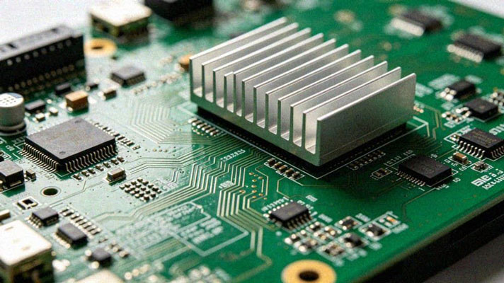
Choosing between them is a stackup decision, and the stackup also fixes the width that produces the required impedance.

Controlled Impedance and How Width Is Calculated

Controlled impedance means the same characteristic impedance along the entire length of the trace. A mismatch in the middle produces a reflection and a disturbance in the received data. To hold the impedance, the designer calculates the trace width from the dielectric thickness, the dielectric constant and the copper thickness, and then uses that width consistently on the layer where it was calculated.

The width can be obtained from a field solver, from the impedance calculator built into most layout tools, or from the fabricator, who can supply both the value and the stackup that produces it. The last option is usually the most reliable for production, because the fabricator knows the actual prepreg thickness after lamination. Whichever route is used, the calculation must be repeated if the stackup changes, and microstrip and stripline routing widths are not interchangeable.

Return Path Integrity

The return current does not simply choose the shortest path to ground; it follows the path of least impedance, which at high frequency means directly beneath the signal trace in the reference plane. Anything that interrupts that plane forces the return current to take a detour, which increases the loop area, adds inductance and radiates.

Splits, slots, connector keep-outs and plane cut-outs are therefore electrical features, not mechanical ones. A signal that crosses a plane split has an uncontrolled return path and no defined impedance. When a crossing is unavoidable, in these high-frequency trace and data bus routing situations, a stitching capacitor placed close to the crossing provides a local return path, but the better answer is usually to move the signal or change the plane.

Routing Rules for Transmission Lines

Keep a transmission line on one layer for as much of its length as possible. Every transition between layers adds a via, and every via adds a discontinuity and, if it passes through the plane, a stub that resonates at some frequency. Where a transition is necessary, use a via whose depth matches the transition, or back-drill the stub, and place ground vias adjacent to it so the return current can follow.

Do not route transmission lines through crowded areas where the reference plane is perforated by anti-pads. The anti-pads of other vias create a mesh of copper that no longer looks like a solid plane at high frequency, and the impedance rises. Where a line has to pass close to other signals, spacing of at least three times the trace width reduces coupling, which is why the 3W crosstalk rule remains a useful default.

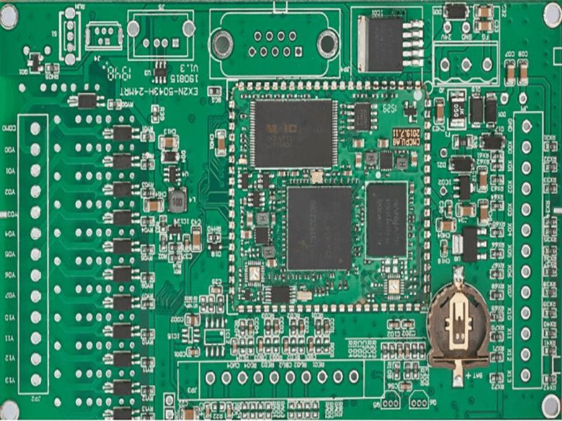
Differential pairs add a second conductor to the problem and change some of the rules.

Differential Pair Considerations

A differential pair is a transmission line with two conductors whose impedances are defined both to the reference plane and to each other. The two traces should be routed together with a constant gap, and the pair should not be separated to pass around a via, a connector pin or a component. Any place where the spacing changes is an impedance discontinuity, and the mismatch between the two traces converts part of the differential signal into common mode noise.

Intra-pair skew is as important as impedance. If one trace of the pair is longer than the other, the differential signal is degraded and common mode energy increases. Length matching should be done at the point where the skew is introduced, with tuning patterns that keep the coupled sections compact, and the pair-to-plane spacing should be smaller than the pair-to-pair spacing so coupling stays within the pair.

Verification

Checking transmission line design is partly analytical and partly empirical. Field solving the critical nets before layout sign-off catches the obvious impedance and coupling problems. After fabrication, time-domain reflectometry on test coupons confirms that the as-built impedance matches the target, and eye diagram measurements on the assembled board show whether the link has margin left.

The value of the earlier work is that it turns a design from something that happens to work into something that can be reproduced. Transmission line behaviour is predictable, and treating it as such is what separates a high-speed layout that passes on the first build from one that needs three revisions.

FAQ

Is microstrip or stripline better for high-speed signals? Stripline gives better impedance stability and lower radiation, while microstrip is easier to route and to probe. Most boards use microstrip on the outer layers and stripline for the fastest nets on inner layers.

How long can a trace be before it behaves as a transmission line? There is no fixed length. Compare the one-way propagation delay with the signal rise time: when the delay becomes a significant fraction of the rise time, transmission line behaviour dominates.

Do I need controlled impedance if the trace is short? Not necessarily. Short nets whose delay is a small fraction of the rise time behave as lumped connections. Controlled impedance earns its cost on long nets and fast edges.