Insertion Loss In High Speed PCB Traces

A long high speed link does not fail because the driver is too weak or the receiver too insensitive. It fails because the channel has quietly removed the high frequency content that the receiver needed to resolve a one from a zero, and by the time the eye closes the damage is distributed along the whole trace rather than concentrated at one point.

Insertion loss is the quantity that describes this removal. It is the ratio of the power delivered to the far end of a channel to the power launched into it, expressed in decibels, and it rises with frequency. Understanding which part of it comes from the copper, which from the laminate, and which from the connectors and vias is what allows a loss budget to be built before the layout is frozen.

What The Measurement Describes

Insertion loss is measured by launching a swept signal into one end of a channel and measuring what arrives at the other, with both ports referenced to the same impedance. The result is a curve that falls with frequency, and the shape of the curve matters as much as the value at any single point. A channel that is flat to two gigahertz and then falls steeply behaves differently from one that falls gently from the start, even if both have the same value at five gigahertz.

The specification for a serial interface is usually written as a limit on the loss at the Nyquist frequency of the data rate, with a further limit on the integrated loss across the band. For a link running at ten gigabits per second, the Nyquist frequency is five gigahertz, and the channel is typically expected to stay within a defined mask around that point.

Conductor Loss And The Skin Effect

At low frequency, current distributes evenly through the cross section of a trace and the resistance is simply the bulk resistance of copper. As frequency rises, current is pushed toward the surface, and the effective cross section shrinks until only a thin outer layer carries the signal. The depth of that layer falls with the square root of frequency, so the resistance rises in the same proportion.

The practical consequence is that copper loss grows as the square root of frequency while dielectric loss grows linearly, which means the balance between them changes across the band. At moderate rates, copper dominates. Above a few gigahertz on a long trace, the dielectric term usually takes over, and this is why improving surface roughness alone stops helping at some point.

Dielectric Loss And The Laminate

The laminate removes energy every time the field reverses, and the loss tangent of the material is the number that predicts how much. Standard FR-4 has a loss tangent in the range of two hundredths, while materials designed for high speed work are an order of magnitude better. The improvement is not free, and it is not uniform: the low loss materials also differ in dielectric constant, in expansion behaviour and in the process window they need.

Because dielectric loss scales with frequency and with length, it is the term that decides whether a link is feasible at all. Halving the loss tangent doubles the distance a given data rate can travel, which is why a low loss laminate is chosen for backplanes and for long cable-less interconnects rather than for short board-to-board links.

Geometry, Impedance And Loss

Trace geometry sets both the impedance and the loss, and the two cannot be optimised independently. Widening a trace for a given impedance requires a thicker dielectric, which reduces conductor loss but increases the volume of field in the dielectric where the lossy resin sits. Narrowing the trace has the opposite effect. The optimum depends on which loss term dominates at the frequency of interest.

Impedance also determines the current for a given voltage, and therefore the resistive loss directly. A fifty ohm line carrying the same voltage as a seventy five ohm line dissipates more power per unit length, which is part of why lower impedance is not automatically better for a long channel. Selecting the geometry on a field solver with the real material parameters is the only way to compare the two effects honestly.

Vias, Connectors And Everything Else

The trace is only part of the channel. A via presents a short section of higher capacitance and lower impedance whose discontinuity reflects energy, and a connector presents a transition between two transmission line geometries. Both add loss that is concentrated in a short length, which is why they are usually worse than an equivalent length of trace.

Stubs are worse still. An unused via that extends below the layer where the trace leaves the barrel creates a resonant stub whose length determines the frequency at which it begins to remove energy. Back drilling removes the unused portion and is a standard remedy on thick backplanes, and where it is not available, the routing of the high frequency nets should keep the layer transitions as few as the topology allows.

Building The Loss Budget

A loss budget is a table. Each element of the channel contributes a figure at the frequency of interest, and the total is compared with the specification with some margin held back for manufacturing variation. Trace loss is estimated from the material and the geometry, via loss from the number of transitions, connector loss from the vendor’s data, and the package loss from the device datasheet.

The discipline of writing the table is what prevents the surprise. Where the budget shows the link is marginal, the options are visible: reduce the number of vias, shorten the route, change the laminate, or lower the data rate. Discovering the same thing after the board is built removes all four options at once.

Measuring And Verifying

A vector network analyser measures insertion loss directly through a test coupon or a connectorised channel, and the result can be compared with the model. On a production board the coupon is the practical route, because probing a finished trace is difficult without disturbing it. The difference between the model and the measurement is usually the material parameters and the via model rather than the trace geometry.

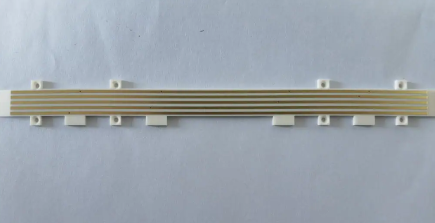
Where a coupon does not exist, a time domain measurement can still identify which part of the channel is responsible. Comparing a trace launched as a microstrip or stripline coupon with the full channel isolates the contribution of the vias and the connectors, and the result feeds back into the next revision of the stackup.

FAQ

Does a wider trace always reduce loss? It reduces conductor loss, but it changes the impedance and the dielectric volume at the same time. On a dielectric dominated channel, a wider trace with a thicker dielectric can measure worse. The comparison has to be made at constant impedance.

How much margin should a loss budget carry? Enough to cover laminate dielectric constant variation and copper roughness variation between fabrication lots. Ten to twenty percent of the allowed loss is a common allowance, and the figure should be stated rather than assumed.

Can a link be equalised instead of shortened? Yes, many high speed interfaces include transmitter and receiver equalisation, which compensates for a predictable loss profile. Equalisation buys margin but it does not create information that the channel has removed, and it will not fix a channel whose loss violates the specification.