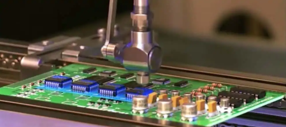
High-Speed Simulation Workflow for PCB Design

High-speed design decisions are expensive to change late, and a high-speed simulation is the cheapest way to make them early. The practical question is not whether to simulate but what to simulate, at which stage and to what accuracy. A workflow that answers those questions produces useful numbers while they can still influence the layout, instead of a report written after the board is routed.

What Has to Be Answered

Four questions dominate high-speed design. How much loss will the channel have, and what does that imply for the maximum usable length? What is the trace impedance and how much does it vary? Where are the resonances in the power delivery network, and is the decoupling sufficient? What coupling or radiation will the finished layout produce? Each question needs a different modelling approach and a different class of tool.

Traditional design rules do not answer them at gigabit rates. Skin effect, dielectric loss, coupling and driver pre-emphasis interact, and a rule of thumb carried over from a slower generation is either too conservative or simply wrong.

Pre-Layout Analysis

A pre-layout analysis sets the constraints before the layout exists. Starting from the topology, the package information and a candidate stackup, a channel simulation estimates skin effect and dielectric loss, then produces the maximum allowed trace length for the data rate, the spacing needed to control coupling, the termination scheme and the maximum intra-pair mismatch. The results become the design rules the router is given.

Doing this first is what makes the constraints realistic. Postponing the analysis until after routing means the constraints were guessed, and a violation discovered at that point forces either a re-route or an accepted risk.

With constraints in place, the next step is to model the loss mechanisms accurately enough to trust the budget.

Loss Budget and Equalization

At multi-gigabit rates the channel loss is dominated by the dielectric at high frequency, with skin effect contributing at lower frequencies. A simulator used for this work must handle lossy transmission lines with frequency-dependent parameters. The output is a loss-versus-frequency curve, and the budget is simply the loss the receiver can tolerate at the Nyquist frequency of the data rate.

Where the budget is tight, equalization and pre-emphasis extend the reach. Passive equalization built from discrete components can be modelled by removing that network from the device model and simulating it on its own. Active equalization inside the driver is harder to represent with a behavioural model, so the analysis may need a transistor-level model before the result can be trusted.

Power Integrity Analysis

The power distribution network is a resonant structure, and its impedance has to stay below a target across a wide frequency range. A plane pair forms a cavity whose resonances depend on the plane dimensions, the dielectric thickness and the dielectric loss. A transmission line mesh model of the plane pair, analysed in the frequency domain, shows where those resonances sit and how much damping the dielectric and the capacitors provide.

Including dielectric loss usually lowers the resonance peaks considerably, and omitting it produces an unnecessarily pessimistic answer that leads to over-design. The target impedance should itself be derived from the current the device actually draws in a differential sense, not from a worst-case assumption, otherwise the analysis will demand more layers and more capacitors than the design needs.

Device models and geometry-specific effects are the two areas where a general model is not sufficient.

Device Model Verification

Board-level simulation usually relies on behavioural input and output buffer models, which are convenient but not universally accurate. At the highest rates the behavioural model loses validity, and a transistor-level model is required to evaluate a new device. Those models come with package effects and loading conditions, and they should be obtained from the manufacturer and adapted to the actual application.

Once device behaviour is confirmed, the behavioural model used for board-level work can be created and validated against it. Validating a model against another model is not sufficient; a measurement on a test board is the only real confirmation.

Field Solving for Discontinuities

Vias, connectors and package transitions are the parts of a channel that a transmission line model cannot represent. A two-dimensional or three-dimensional field solver extracts the parasitic parameters of these structures, which are then included in the channel simulation. Because the geometry is complex, this work is expensive, so it is applied to the few structures that matter rather than to the whole board.

The results also feed back into the layout as rules: a maximum via stub length, a connector pin assignment that keeps the return path close, or a keep-out around a transition to preserve the reference plane.

Post-Route Verification

After routing, the real geometry is extracted and simulated again. Crosstalk, actual trace lengths and real reference plane gaps are now known, so earlier estimates can be replaced with computed values. This is also where the eye diagram is evaluated with a worst-case data pattern, because a simple clock pattern hides the data-dependent effects that dominate at gigabit rates. Clearing the resulting constraints on high-frequency traces and data buses is a separate review step, not something the router does automatically.

The same extracted model can be reused for emissions work. Once the geometry is known, the coupling between nets and the fields around the board can be evaluated, and the results inform the EMI suppression principles that apply to connectors, cables and the plane structure. Running both analyses from one extraction is far cheaper than building a second model later.

Putting the Workflow Together

The sequence is straightforward. Build the channel model and derive the layout constraints. Model the loss and confirm that the equalization scheme closes the budget. Analyse the power delivery network and set the decoupling requirement. Field-solve the critical discontinuities. Then verify the finished layout against the constraints derived at the start. Each step produces a rule that the layout can be measured against, and the loop is closed by measurement on the first prototypes.

Two practical details decide whether the flow works. First, the models must be versioned together with the layout, because a simulation run against an old stackup proves nothing about the current board. Second, the analysis has to produce numbers that the layout can satisfy, which means the accuracy of each stage should match the decision it supports; a rough estimate is enough for a constraint, while a sign-off check needs the full model. The differences between a microstrip and stripline routing approach illustrate why the stackup has to be fixed before those numbers are generated.

FAQ

Do I need a field solver for every design? No. Field solving is justified for the vias, connectors and transitions on the fastest channels. Below roughly 5 Gbps, analytical models and impedance calculations usually cover the requirement.

Can a behavioural model be used at 10 Gbps and above? It becomes unreliable. At those rates a transistor-level model is normally needed to evaluate a new device, with the behavioural model derived from it for board-level simulation.

When should post-route verification happen? Before the design is released for fabrication, and again if the routing changes materially. A check on an outdated database is worse than no check, because it gives false confidence.