Signal And Power Integrity Analysis Basics
Signal integrity and power integrity are usually treated as two subjects, and on a board they are one. A driver switches current out of the power distribution network and back into it through the ground plane, and the quality of that supply at the moment of switching determines the shape of the edge that leaves the driver. Analysing one without the other produces a model that matches neither.
This article covers the practical sequence of an integrity analysis: what to model, what to measure, and which results indicate a design change rather than a modelling detail.
The analysis is worth doing at the point where the layout still has freedom. Later, the same findings become a list of changes that cannot be made.
What Signal Integrity Analysis Answers
Signal integrity asks whether the waveform arriving at the receiver can be sampled correctly. The relevant quantities are the impedance profile along the channel, the loss, the crosstalk from neighbouring nets, and the timing of the arrival relative to the sampling point. Each has a measurement and a simulation counterpart, and a useful analysis compares the two rather than relying on either alone.
The channel is the unit of analysis, from the driver output through the package, the trace, the vias, the connector and back into the receiver. Modelling only the board trace and ignoring the package is a common simplification that hides the largest single discontinuity in the path on a fast interface.

What Power Integrity Analysis Answers
Power integrity asks whether the voltage at the device pin stays within the tolerance window while the device switches. The quantity that organises the analysis is the target impedance, calculated from the permitted voltage ripple and the current step the device will draw. The power distribution network must present an impedance below that target across the whole frequency range of the switching activity.
The network is a series of elements: the regulator, the bulk capacitors, the ceramic capacitors, the plane pair and the vias connecting them. Each element is effective in its own frequency band, and the design goal is a network whose impedance is below the target everywhere, without a resonance that rises above it between the bands.
Decoupling And Where It Stops Working
A decoupling capacitor is only as good as its connection. The inductance of the vias and the trace between the capacitor and the device pin sets the frequency above which the capacitor no longer helps, and that inductance is usually larger than the capacitor’s own. This is why several small capacitors placed close to the pins outperform one large capacitor at the edge of the board.
The plane pair acts as a distributed capacitance that takes over above the frequency where the discrete capacitors stop being effective. Its behaviour depends on the dielectric thickness between the planes and on the extent of the copper, and it forms resonances whose frequencies depend on the board dimensions. Where a resonance coincides with a switching harmonic, the voltage at the pins can be much worse than the target impedance would suggest.
Plane Resonance And How To Damp It
A power and ground plane pair forms a cavity with resonant modes, and the impedance at resonance can be tens of times higher than the target. The modes depend on the shape and size of the board, so the same stackup on a larger board has its resonances at different frequencies.
Damping is achieved by adding loss. A resistor in series with a capacitor between the planes converts the resonance into a broader, lower peak, and spreading capacitors of different values across the board broadens the response in the same way. Where the planes must be split for different supplies, the rules for splitting power planes also matter, because a split creates a boundary condition that shifts the resonances and can create a path for one rail’s noise to appear on another.
The frequency range of interest is set by the fastest edge in the design, not by the clock. A device that switches a rail in a few nanoseconds excites the network up to several hundred megahertz, and a design whose decoupling was chosen for the switching frequency alone will be short of capacitance exactly where it is needed. Deciding the upper frequency limit of the analysis is therefore the first step, and it should be derived from the edge rate.
Crosstalk And The Mixed Signal Boundary
Crosstalk is analysed as coupled voltage, but the mechanism to keep in mind is shared return current. Two signals that share a return path through the plane couple through the impedance of that path, and the coupling is proportional to the rate of change of current rather than to the voltage on the aggressor.
Where a design contains both analogue and digital circuits, the analysis has to include the reference treatment at the boundary. Following mixed signal design practice keeps the two return currents from sharing a path, which is what prevents the switching noise from appearing as an offset in the measurement.
Simulation, Measurement And Their Disagreement
A simulation is only as good as its inputs. Dielectric constant, loss tangent, copper roughness and via models are all approximations, and the differences accumulate along a long channel. Where a simulation and a measurement disagree, the useful question is which parameter would have to change to explain the difference, and whether that parameter is within its manufacturing range.
Measurement provides the ground truth but is limited by the instrument and the probe. A measurement made with a long ground lead includes the lead in the result, and one made without a calibrated reference includes the cable. Setting up the measurement properly is as important as building the model, and the effort is repaid the first time a marginal result has to be explained.
Sequence For A Practical Analysis
Start with the interfaces that are marginal by inspection: the fastest link, the highest current device, the longest route. Model the full channel for those, and measure the same channel on a coupon or a prototype where one is available. Then check the plane resonances against the switching spectrum, and confirm that the decoupling network is below the target impedance across the band.
Finally, confirm the structural assumptions that the whole analysis rests on: reference plane continuity, the stackup used to control emissions, and the via transitions that connect the layers. A model built on a stackup that the fabricator did not build is a model of a different board.
Documentation is the last element of a useful analysis. The assumptions, the material parameters used, the measurement setup and the discrepancy between model and measurement should be recorded in one place, because the next revision will start from them. An analysis whose inputs are lost is an analysis that has to be repeated in full the next time the board is changed.
FAQ
Which should be analysed first, signal or power integrity? Power integrity, in practice, because the supply sets the edge that signal integrity then propagates. An output that is not well supplied produces a waveform that no amount of trace tuning will repair.
How accurate does the loss tangent need to be? Accurate enough to be inside the manufacturing spread of the material. Where the supplier gives a range, the analysis should be run at both ends of the range rather than at the typical value.
Can a design pass simulation and fail in the lab? Frequently, and the usual causes are the package model, the connector, and the assumption that the reference plane is continuous. These are the three items worth verifying physically before trusting the simulation.